Breaking Linear Classifiers on ImageNet
You’ve probably heard that Convolutional Networks work very well in practice and across a wide range of visual recognition problems. You may have also read articles and papers that claim to reach a near “human-level performance”. There are all kinds of caveats to that (e.g. see my G+ post on Human Accuracy is not a point, it lives on a tradeoff curve), but that is not the point of this post. I do think that these systems now work extremely well across many visual recognition tasks, especially ones that can be posed as simple classification.
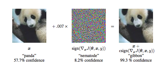
Yet, a second group of seemingly baffling results has emerged that brings up an apparent contradiction. I’m referring to several people who have noticed that it is possible to take an image that a state-of-the-art Convolutional Network thinks is one class (e.g. “panda”), and it is possible to change it almost imperceptibly to the human eye in such a way that the Convolutional Network suddenly classifies the image as any other class of choice (e.g. “gibbon”). We say that we break, or fool ConvNets. See the image below for an illustration:
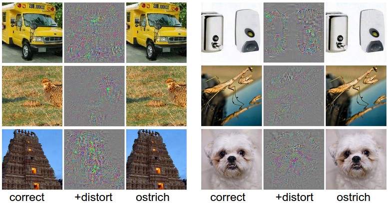
This topic has recently gained attention starting with Intriguing properties of neural networks by Szegedy et al. last year. They had a very similar set of images:
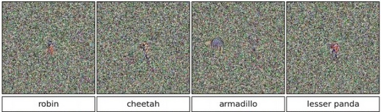
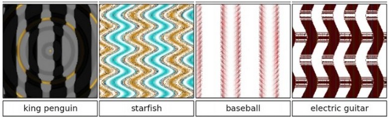
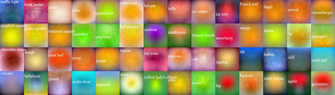
And a set of very closely related results was later followed by Deep Neural Networks are Easily Fooled: High Confidence Predictions for Unrecognizable Images by Nguyen et al. Instead of starting with correctly-classified images and fooling the ConvNet, they had many more examples of performing the same process starting from noise (and hence making the ConvNet confidently classify an incomprehensible noise pattern as some class), or evolving new funny-looking images that the ConvNet is slightly too certain about:
I should make the point quickly that these results are not completely new to Computer Vision, and that some have observed the same problems even with our older features, e.g. HOG features. See Exploring the Representation Capabilities of the HOG Descriptor for details.
The conclusion seems to be that we can take any arbitrary image and classify it as whatever class we want by adding tiny, imperceptible noise patterns. Worse, it was found that a reasonable fraction of fooling images generalize across different Convolutional Networks, so this isn’t some kind of fragile property of the new image or some overfitting property of the model. There’s something more general about the type of introduced noise that seems to fool many other models. In some sense, it is much more accurate to speak about fooling subspaces rather than fooling images. The latter erroneously makes them seem like tiny points in the super-high-dimensional image space, perhaps similar to rational numbers along the real numbers, when instead they are better thought of as entire intervals. Of course, this work raises security concerns because an adversary could conceivably generate a fooling image of any class on their own computer and upload it to some service with a malicious intent, with a non-zero probability of it fooling the server-side model (e.g. circumventing racy filters).
What is going on?
These results are interesting and worrying, but they have also led to a good amount of confusion among laymen. The most important point of this entire post is the following:
These results are not specific to images, ConvNets, and they are also not a “flaw” in Deep Learning. A lot of these results were reported with ConvNets running on images because pictures are fun to look at and ConvNets are state-of-the-art, but in fact the core flaw extends to many other domains (e.g. speech recognition systems), and most importantly, also to simple, shallow, good old-fashioned Linear Classifiers (Softmax classifier, or Linear Support Vector Machines, etc.). This was pointed out and articulated in Explaining and Harnessing Adversarial Examples by Goodfellow et al. We’ll carry out a few experiments very similar to the ones presented in this paper, and see that it is in fact this linear nature that is problematic. And because Deep Learning models use linear functions to build up the architecture, they inherit their flaw. However, Deep Learning by itself is not the cause of the issue. In fact, Deep Learning offers tangible hope for a solution, since we can use all the wiggle of composed functions to design more resistant architectures or objectives.
How fooling methods work
ConvNets express a differentiable function from the pixel values to class scores. For example, a ConvNet might take a 227x227 image and transforms these ~100,000 numbers through a wiggly function (parameterized by several million parameters) to 1000 numbers that we interpret as the confidences for 1000 classes (e.g. the classes of ImageNet).
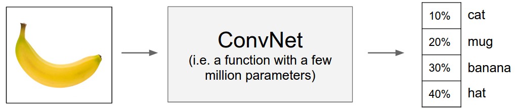
We train a ConvNet with repeated process of sampling data, calculating the parameter gradients and performing a parameter update. That is, suppose we feed the ConvNet an image of a banana and compute the 1000 scores for the classes that the ConvNet assigns to this image. We then and ask the following question for every single parameter in the model:
Normal ConvNet training: “What happens to the score of the correct class when I wiggle this parameter?”
This wiggle influence, of course, is just the gradient. For example, some parameter in some filter in some layer of the ConvNet might get the gradient of -3.0 computed during backpropagation. That means that increasing this parameter by a tiny amount, e.g. 0.0001, would have a negative influence on the banana score (due to the negative sign); In this case, we’d expect the banana score to decrease by approximately 0.0003. Normally we take this gradient and use it to perform a parameter update, which wiggles every parameter in the model a tiny amount in the correct direction, to increase the banana score. These parameter updates hence work in concert to slightly increase the score of the banana class for that one banana image (e.g. the banana score could go up from 30% to 34% or something). We then repeat this over and over on all images in the training data.
Notice how this worked: we held the input image fixed, and we wiggled the model parameters to increase the score of whatever class we wanted (e.g. banana class). It turns out that we can easily flip this process around to create fooling images. (In practice in fact, absolutely no changes to a ConvNet code base are required.) That is, we will hold the model parameters fixed, and instead we’re computing the gradient of all pixels in the input image on any class we might desire. For example, we can ask:
Creating fooling images: “What happens to the score of (whatever class you want) when I wiggle this pixel?”
We compute the gradient just as before with backpropagation, and then we can perform an image update instead of a parameter update, with the end result being that we increase the score of whatever class we want. E.g. we can take the banana image and wiggle every pixel according to the gradient of that image on the cat class. This would change the image a tiny amount, but the score of cat would now increase. Somewhat unintuitively, it turns out that you don’t have to change the image too much to toggle the image from being classified correctly as a banana, to being classified as anything else (e.g. cat).
In short, to create a fooling image we start from whatever image we want (an actual image, or even a noise pattern), and then use backpropagation to compute the gradient of the image pixels on any class score, and nudge it along. We may, but do not have to, repeat the process a few times. You can interpret backpropagation in this setting as using dynamic programming to compute the most damaging local perturbation to the input. Note that this process is very efficient and takes negligible time if you have access to the parameters of the ConvNet (backprop is fast), but it is possible to do this even if you do not have access to the parameters but only to the class scores at the end. In this case, it is possible to compute the data gradient numerically, or to to use other local stochastic search strategies, etc. Note that due to the latter approach, even non-differentiable classifiers (e.g. Random Forests) are not safe (but I haven’t seen anyone empirically confirm this yet).
Fooling a Linear Classifier on ImageNet
As I mentioned before (and as described in more detail in Goodfellow et al.), it is the use of linear functions that makes our models susceptible for an attack. ConvNets, of course, do not express a linear function from images to class scores; They are a complex Deep Learning model that expresses a highly non-linear function. However, the components that make up a ConvNet are linear: Convolution of a filter with its input is a linear operation (we are sliding a filter through the input and computing dot products - a linear operation), and matrix multiplications are also a linear function.
So here’s a fun experiment we’ll do. Lets forget about ConvNets - they are a distracting overkill as far as the core flaw goes. Instead, lets fool a linear classifier and lets also keep with the theme of breaking models on images because they are fun to look at.
Here is the setup:
- Take 1.2 million images in ImageNet
- Resize them to 64x64 (full-sized images would train longer)
- use Caffe to train a Linear Classifier (e.g. Softmax). In other words we’re going straight from data to the classifier with a single fully-connected layer.
Digression: Technical fun parts. The fun part in actually doing this is that the standard AlexNetty ConvNet hyperparameters are of course completely inadequate. For example, normally you’d use weight decay of 0.0005 or so and learning rate of 0.01, and gaussian initialization drawn from a gaussian of 0.01 std. If you’ve trained linear classifiers before on this type of high-dimensional input (64x64x3 ~= 12K numbers), you’ll know that your learning rate will probably have to be much lower, the regularization much larger, and initialization of 0.01 std will probably be inadequate. Indeed, starting Caffe training with default hyperparameters gives a starting loss of about 80, which right away tells you that the initialization is completely out of whack (initial ImageNet loss should be ballpark 7.0, which is -log(1/1000)). I scaled it down to 0.0001 std for Gaussian init which gives sensible starting loss. But then the loss right away explodes which tells you that the learning rate is way too high - I had to scale it all the way down to about 1e-7. Lastly, a weight decay of 0.0005 will give almost negligible regularization loss with 12K inputs - I had to scale it up to 100 to start getting reasonably-looking weights that aren’t super-overfitted noise blobs. It’s fun being a Neural Networks practitioner.
A linear classifier over image pixels implies that every class score is computed as a dot product between all the image pixels (stretched as a large column) and a learnable weight vector, one for each class. With input images of size 64x64x3 and 1000 ImageNet classes we therefore have 64x64x3x1000 = 12.3 million weights (beefy linear model!), and 1000 biases. Training these parameters on ImageNet with a K40 GPU takes only a few tens of minutes. We can then visualize each of the learned weights by reshaping them as images:
By the way, I haven’t seen anyone report linear classification accuracy on ImageNet before, but it turns out to be about 3.0% top-1 accuracy (and about 10% top-5) on ImageNet. I haven’t done a completely exhaustive hyperparameter sweep but I did a few rounds of manual binary search.
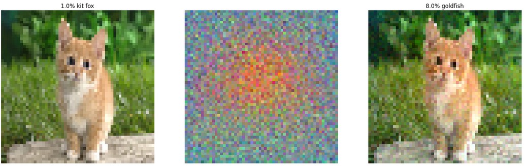
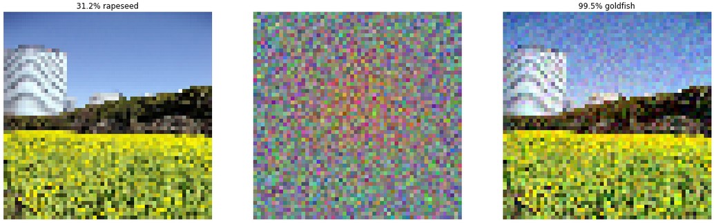
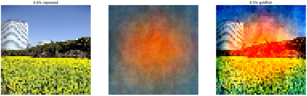
Now that we’ve trained the model parameters we can start to produce fooling images. This turns out to be quite trivial in the case of linear classifiers and no backpropagation is required. This is because when your score function is a dot product \(s = w^Tx\), then the gradient on the image \(x\) is simply \(\nabla_x s = w\). That is, we take an image we would like to start out with, and then if we wanted to fool the model into thinking that it is some other class (e.g. goldfish), we have to take the weights corresponding to the desired class, and add some fraction of those weights to the image:
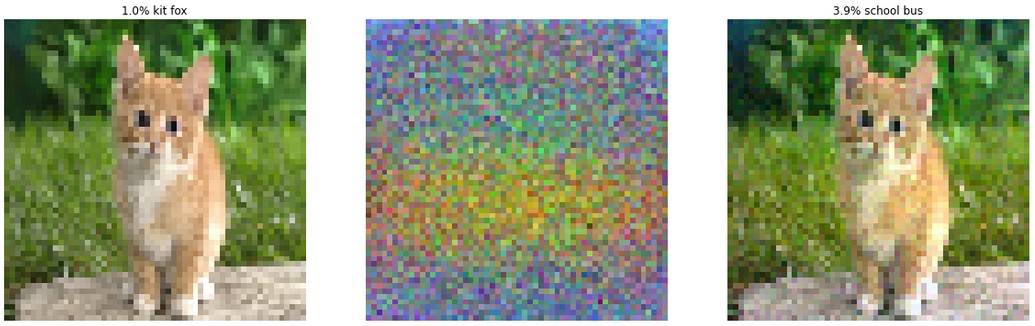
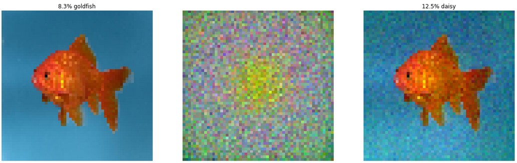
We can also start from random noise and achieve the same effect:
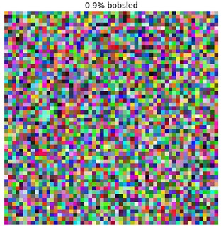
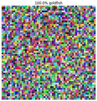
Of course, these examples are not as impactful as the ones that use a ConvNet because the ConvNet gives state of the art performance while a linear classifier barely gets to 3% accuracy, but it illustrates the point that even with a simple, shallow function it is still possible to play around with the input in imperceptible ways and get almost arbitrary results.
Regularization. There is one subtle comment to make regarding regularization strength. In my experiments above, increasing the regularization strength gave nicer, smoother and more diffuse weights but generalized to validation data worse than some of my best classifiers that displayed more noisy patterns. For example, the nice and smooth templates I’ve shown only achieve 1.6% accuracy. My best model that achieves 3.0% accuracy has noisier weights (as seen in the middle column of the fooling images). Another model with very low regularization reaches 2.8% and its fooling images are virtually indistinguishable yet produce 100% confidences in the wrong class. In particular:
- High regularization gives smoother templates, but at some point starts to works worse. However, it is more resistant to fooling. (The fooling images look noticeably different from their original)
- Low regularization gives more noisy templates but seems to work better that all-smooth templates. It is less resistant to fooling.
Intuitively, it seems that higher regularization leads to smaller weights, which means that one must change the image more dramatically to change the score by some amount. It’s not immediately obvious if and how this conclusion translates to deeper models.
Toy Example
We can understand this process in even more detail by condensing the problem to the smallest toy example that displays the problem. Suppose we train a binary logistic regression, where we define the probability of class 1 as \(P(y = 1 \mid x; w,b) = \sigma(w^Tx + b)\), where \(\sigma(z) = 1/(1+e^{-z})\) is the sigmoid function that squashes the class 1 score \(s = w^Tx+b\) into range between 0 and 1, where 0 is mapped to 0.5. This classifier hence decides that the class of the input is 1 if \(s > 0\), or equivalently if the class 1 probability is more than 50% (i.e. \(\sigma(s) > 0.5\)). Suppose further that we had the following setup:
x = [2, -1, 3, -2, 2, 2, 1, -4, 5, 1] // input
w = [-1, -1, 1, -1, 1, -1, 1, 1, -1, 1] // weight vector
If you do the dot product, you get -3. Hence, probability of class 1 is 1/(1+e^(-(-3))) = 0.0474. In other words the classifier is 95% certain that this is example is class 0. We’re now going to try to fool the classifier. That is, we want to find a tiny change to x in such a way that the score comes out much higher. Since the score is computed with a dot product (multiply corresponding elements in x and w then add it all up), with a little bit of thought it’s clear what this change should be: In every dimension where the weight is positive, we want to slightly increase the input (to get slightly more score). Conversely, in every dimension where the weight is negative, we want the input to be slightly lower (again, to get slightly more score). In other words, an adversarial xad might be:
// xad = x + 0.5w gives:
xad = [1.5, -1.5, 3.5, -2.5, 2.5, 1.5, 1.5, -3.5, 4.5, 1.5]
Doing the dot product again we see that suddenly the score becomes 2. This is not surprising: There are 10 dimensions and we’ve tweaked the input by 0.5 in every dimension in such a way that we gain 0.5 in each one, adding up to a total of 5 additional score, rising it from -3 to 2. Now when we look at probability of class 1 we get 1/(1+e^(-2)) = 0.88. That is, we tweaked the original x by a small amount and we improved the class 1 probability from 5% to 88%! Moreover, notice that in this case the input only had 10 dimensions, but an image might consist of many tens of thousands of dimensions, so you can afford to make tiny changes across all of them that all add up in concert in exactly the worst way to blow up the score of any class you wish.
Conclusions
Several other related experiments can be found in Explaining and Harnessing Adversarial Examples by Goodfellow et al. This paper is a required reading on this topic. It was the first to articulate and point out the linear functions flaw, and more generally argued that there is a tension between models that are easy to train (e.g. models that use linear functions) and models that resist adversarial perturbations.
As closing words for this post, the takeaway is that ConvNets still work very well in practice. Unfortunately, it seems that their competence is relatively limited to a small region around the data manifold that contains natural-looking images and distributions, and that once we artificially push images away from this manifold by computing noise patterns with backpropagation, we stumble into parts of image space where all bets are off, and where the linear functions in the network induce large subspaces of fooling inputs.
With wishful thinking, one might hope that ConvNets would produce all-diffuse probabilities in regions outside the training data, but there is no part in an ordinary objective (e.g. mean cross-entropy loss) that explicitly enforces this constraint. Indeed, it seems that the class scores in these regions of space are all over the place, and worse, a straight-forward attempt to patch this up by introducing a background class and iteratively adding fooling images as a new background class during training are not effective in mitigating the problem.
It seems that to fix this problem we need to change our objectives, our forward functional forms, or even the way we optimize our models. However, as far as I know we haven’t found very good candidates for either. To be continued.
Further Reading
- Ian Goodfellow gave a talk on this work at the RE.WORK Deep Learning Summit 2015
- You can fool ConvNets as part of CS231n Assignment #3 IPython Notebook.
- IPython Notebook for this experiment. Also my Caffe linear classifier protos if you like.