Deep Neural Nets: 33 years ago and 33 years from now
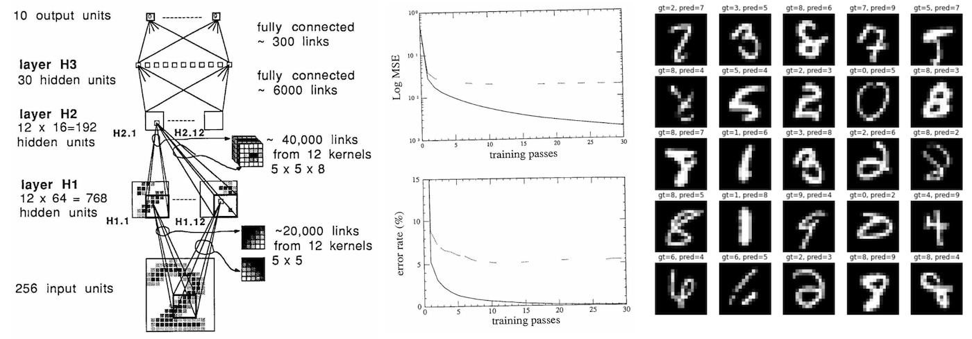
The Yann LeCun et al. (1989) paper Backpropagation Applied to Handwritten Zip Code Recognition is I believe of some historical significance because it is, to my knowledge, the earliest real-world application of a neural net trained end-to-end with backpropagation. Except for the tiny dataset (7291 16x16 grayscale images of digits) and the tiny neural network used (only 1,000 neurons), this paper reads remarkably modern today, 33 years later - it lays out a dataset, describes the neural net architecture, loss function, optimization, and reports the experimental classification error rates over training and test sets. It’s all very recognizable and type checks as a modern deep learning paper, except it is from 33 years ago. So I set out to reproduce the paper 1) for fun, but 2) to use the exercise as a case study on the nature of progress in deep learning.
Implementation. I tried to follow the paper as close as possible and re-implemented everything in PyTorch in this karpathy/lecun1989-repro github repo. The original network was implemented in Lisp using the Bottou and LeCun 1988 backpropagation simulator SN (later named Lush). The paper is in french so I can’t super read it, but from the syntax it looks like you can specify neural nets using higher-level API similar to what you’d do in something like PyTorch today. As a quick note on software design, modern libraries have adopted a design that splits into 3 components: 1) a fast (C/CUDA) general Tensor library that implements basic mathematical operations over multi-dimensional tensors, and 2) an autograd engine that tracks the forward compute graph and can generate operations for the backward pass, and 3) a scriptable (Python) deep-learning-aware, high-level API of common deep learning operations, layers, architectures, optimizers, loss functions, etc.
Training. During the course of training we have to make 23 passes over the training set of 7291 examples, for a total of 167,693 presentations of (example, label) to the neural network. The original network trained for 3 days on a SUN-4/260 workstation. I ran my implementation on my MacBook Air (M1) CPU, which crunched through it in about 90 seconds (~3000X naive speedup). My conda is setup to use the native arm64 builds, rather than Rosetta emulation. The speedup may have been more dramatic if PyTorch had support for the full capability of the M1 (including the GPU and the NPU), but this seems to still be in development. I also tried naively running the code on an A100 GPU, but the training was actually slower, most likely because the network is so tiny (4 layer convnet with up to 12 channels, total of 9760 params, 64K MACs, 1K activations), and the SGD uses only a single example at a time. That said, if one really wanted to crush this problem with modern hardware (A100) and software infrastructure (CUDA, PyTorch), we’d need to trade per-example SGD for full-batch training to maximize GPU utilization and most likely achieve another ~100X speedup of training latency.
Reproducing 1989 performance. The original paper reports the following results:
eval: split train. loss 2.5e-3. error 0.14%. misses: 10
eval: split test . loss 1.8e-2. error 5.00%. misses: 102
While my training script repro.py in its current form prints at the end of the 23rd pass:
eval: split train. loss 4.073383e-03. error 0.62%. misses: 45
eval: split test . loss 2.838382e-02. error 4.09%. misses: 82
So I am reproducing the numbers roughly, but not exactly. Sadly, an exact reproduction is most likely not possible because the original dataset has, I believe, been lost to time. Instead, I had to simulate it using the larger MNIST dataset (hah never thought I’d say that) by taking its 28x28 digits, scaling them down to 16x16 pixels with bilinear interpolation, and randomly without replacement drawing the correct number of training and test set examples from it. But I am sure there are other culprits at play. For example, the paper is a bit too abstract in its description of the weight initialization scheme, and I suspect that there are some formatting errors in the pdf file that, for example, erase dots “.”, making “2.5” look like like “2 5”, and potentially (I think?) erasing square roots. E.g. we’re told that the weight init is drawn from uniform “2 4 / F” where F is the fan-in, but I am guessing this surely (?) means “2.4 / sqrt(F)”, where the sqrt helps preserve the standard deviation of outputs. The specific sparse connectivity structure between the H1 and H2 layers of the net are also brushed over, the paper just says it is “chosen according to a scheme that will not be discussed here”, so I had to make some some sensible guesses here with an overlapping block sparse structure. The paper also claims to use tanh non-linearity, but I am worried this may have actually been the “normalized tanh” that maps ntanh(1) = 1, and potentially with an added scaled-down skip connection, which was trendy at the time to ensure there is at least a bit of gradient in the flat tails of the tanh. Lastly, the paper uses a “special version of Newton’s algorithm that uses a positive, diagonal approximation of Hessian”, but I only used SGD because it is significantly simpler and, according to the paper, “this algorithm is not believed to bring a tremendous increase in learning speed”.
Cheating with time travel. Around this point came my favorite part. We are living here 33 years in the future and deep learning is a highly active area of research. How much can we improve on the original result using our modern understanding and 33 years of R&D? My original result was:
eval: split train. loss 4.073383e-03. error 0.62%. misses: 45
eval: split test . loss 2.838382e-02. error 4.09%. misses: 82
The first thing I was a bit sketched out about is that we are doing simple classification into 10 categories, but at the time this was modeled as a mean squared error (MSE) regression into targets -1 (for negative class) or +1 (for positive class), with output neurons that also had the tanh non-linearity. So I deleted the tanh on output layers to get class logits and swapped in the standard (multiclass) cross entropy loss function. This change dramatically improved the training error, completely overfitting the training set:
eval: split train. loss 9.536698e-06. error 0.00%. misses: 0
eval: split test . loss 9.536698e-06. error 4.38%. misses: 87
I suspect one has to be much more careful with weight initialization details if your output layer has the (saturating) tanh non-linearity and an MSE error on top of it. Next, in my experience a very finely-tuned SGD can work very well, but the modern Adam optimizer (learning rate of 3e-4, of course :)) is almost always a strong baseline and needs little to no tuning. So to improve my confidence that optimization was not holding back performance, I switched to AdamW with LR 3e-4, and decay it down to 1e-4 over the course of training, giving:
eval: split train. loss 0.000000e+00. error 0.00%. misses: 0
eval: split test . loss 0.000000e+00. error 3.59%. misses: 72
This gave a slightly improved result on top of SGD, except we also have to remember that a little bit of weight decay came in for the ride as well via the default parameters, which helps fight the overfitting situation. As we are still heavily overfitting, next I introduced a simple data augmentation strategy where I shift the input images by up to 1 pixel horizontally or vertically. However, because this simulates an increase in the size of the dataset, I also had to increase the number of passes from 23 to 60 (I verified that just naively increasing passes in original setting did not substantially improve results):
eval: split train. loss 8.780676e-04. error 1.70%. misses: 123
eval: split test . loss 8.780676e-04. error 2.19%. misses: 43
As can be seen in the test error, that helped quite a bit! Data augmentation is a fairly simple and very standard concept used to fight overfitting, but I didn’t see it mentioned in the 1989 paper, perhaps it was a more recent innovation (?). Since we are still overfitting a bit, I reached for another modern tool in the toolbox, Dropout. I added a weak dropout of 0.25 just before the layer with the largest number of parameters (H3). Because dropout sets activations to zero, it doesn’t make as much sense to use it with tanh that has an active range of [-1,1], so I swapped all non-linearities to the much simpler ReLU activation function as well. Because dropout introduces even more noise during training, we also have to train longer, bumping up to 80 passes, but giving:
eval: split train. loss 2.601336e-03. error 1.47%. misses: 106
eval: split test . loss 2.601336e-03. error 1.59%. misses: 32
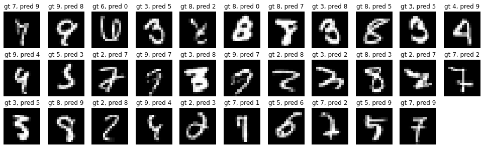
Which brings us down to only 32 / 2007 mistakes on the test set! I verified that just swapping tanh -> relu in the original network did not give substantial gains, so most of the improvement here is coming from the addition of dropout. In summary, if I time traveled to 1989 I’d be able to cut the rate of errors by about 60%, taking us from ~80 to ~30 mistakes, and an overall error rate of ~1.5% on the test set. This gain did not come completely free because we also almost 4X’d the training time, which would have increased the 1989 training time from 3 days to almost 12. But the inference latency would not have been impacted. The remaining errors are here:
Going further. However, after swapping MSE -> Softmax, SGD -> AdamW, adding data augmentation, dropout, and swapping tanh -> relu I’ve started to taper out on the low hanging fruit of ideas. I tried a few more things (e.g. weight normalization), but did not get substantially better results. I also tried to miniaturize a Visual Transformer (ViT)) into a “micro-ViT” that roughly matches the number of parameters and flops, but couldn’t match the performance of a convnet. Of course, many other innovations have been made in the last 33 years, but many of them (e.g. residual connections, layer/batch normalizations) only become relevant in much larger models, and mostly help stabilize large-scale optimization. Further gains at this point would likely have to come from scaling up the size of the network, but this would bloat the test-time inference latency.
Cheating with data. Another approach to improving the performance would have been to scale up the dataset, though this would come at a dollar cost of labeling. Our original reproduction baseline, again for reference, was:
eval: split train. loss 4.073383e-03. error 0.62%. misses: 45
eval: split test . loss 2.838382e-02. error 4.09%. misses: 82
Using the fact that we have all of MNIST available to us, we can simply try scaling up the training set by ~7X (7,291 to 50,000 examples). Leaving the baseline training running for 100 passes already shows some improvement from the added data alone:
eval: split train. loss 1.305315e-02. error 2.03%. misses: 60
eval: split test . loss 1.943992e-02. error 2.74%. misses: 54
But further combining this with the innovations of modern knowledge (described in the previous section) gives the best performance yet:
eval: split train. loss 3.238392e-04. error 1.07%. misses: 31
eval: split test . loss 3.238392e-04. error 1.25%. misses: 24
In summary, simply scaling up the dataset in 1989 would have been an effective way to drive up the performance of the system, at no cost to inference latency.
Reflections. Let’s summarize what we’ve learned as a 2022 time traveler examining state of the art 1989 deep learning tech:
- First of all, not much has changed in 33 years on the macro level. We’re still setting up differentiable neural net architectures made of layers of neurons and optimizing them end-to-end with backpropagation and stochastic gradient descent. Everything reads remarkably familiar, except it is smaller.
- The dataset is a baby by today’s standards: The training set is just 7291 16x16 greyscale images. Today’s vision datasets typically contain a few hundred million high-resolution color images from the web (e.g. Google has JFT-300M, OpenAI CLIP was trained on a 400M), but grow to as large as a small few billion. This is approx. ~1000X pixel information per image (384*384*3/(16*16)) times 100,000X the number of images (1e9/1e4), for a rough 100,000,000X more pixel data at the input.
- The neural net is also a baby: This 1989 net has approx. 9760 params, 64K MACs, and 1K activations. Modern (vision) neural nets are on the scale of small few billion parameters (1,000,000X) and O(~1e12) MACs (~10,000,000X). Natural language models can reach into trillions of parameters.
- A state of the art classifier that took 3 days to train on a workstation now trains in 90 seconds on my fanless laptop (3,000X naive speedup), and further ~100X gains are very likely possible by switching to full-batch optimization and utilizing a GPU.
- I was, in fact, able to tune the model, augmentation, loss function, and the optimization based on modern R&D innovations to cut down the error rate by 60%, while keeping the dataset and the test-time latency of the model unchanged.
- Modest gains were attainable just by scaling up the dataset alone.
- Further significant gains would likely have to come from a larger model, which would require more compute, and additional R&D to help stabilize the training at increasing scales. In particular, if I was transported to 1989, I would have ultimately become upper-bounded in my ability to further improve the system without a bigger computer.
Suppose that the lessons of this exercise remain invariant in time. What does that imply about deep learning of 2022? What would a time traveler from 2055 think about the performance of current networks?
- 2055 neural nets are basically the same as 2022 neural nets on the macro level, except bigger.
- Our datasets and models today look like a joke. Both are somewhere around 10,000,000X larger.
- One can train 2022 state of the art models in ~1 minute by training naively on their personal computing device as a weekend fun project.
- Today’s models are not optimally formulated, and just changing some of the details of the model, loss function, augmentation or the optimizer we can about halve the error.
- Our datasets are too small, and modest gains would come from scaling up the dataset alone.
- Further gains are actually not possible without expanding the computing infrastructure and investing into some R&D on effectively training models on that scale.
But the most important trend I want to comment on is that the whole setting of training a neural network from scratch on some target task (like digit recognition) is quickly becoming outdated due to finetuning, especially with the emergence of foundation models like GPT. These foundation models are trained by only a few institutions with substantial computing resources, and most applications are achieved via lightweight finetuning of part of the network, prompt engineering, or an optional step of data or model distillation into smaller, special-purpose inference networks. I think we should expect this trend to be very much alive, and indeed, intensify. In its most extreme extrapolation, you will not want to train any neural networks at all. In 2055, you will ask a 10,000,000X-sized neural net megabrain to perform some task by speaking (or thinking) to it in English. And if you ask nicely enough, it will oblige. Yes you could train a neural net too… but why would you?