microgpt
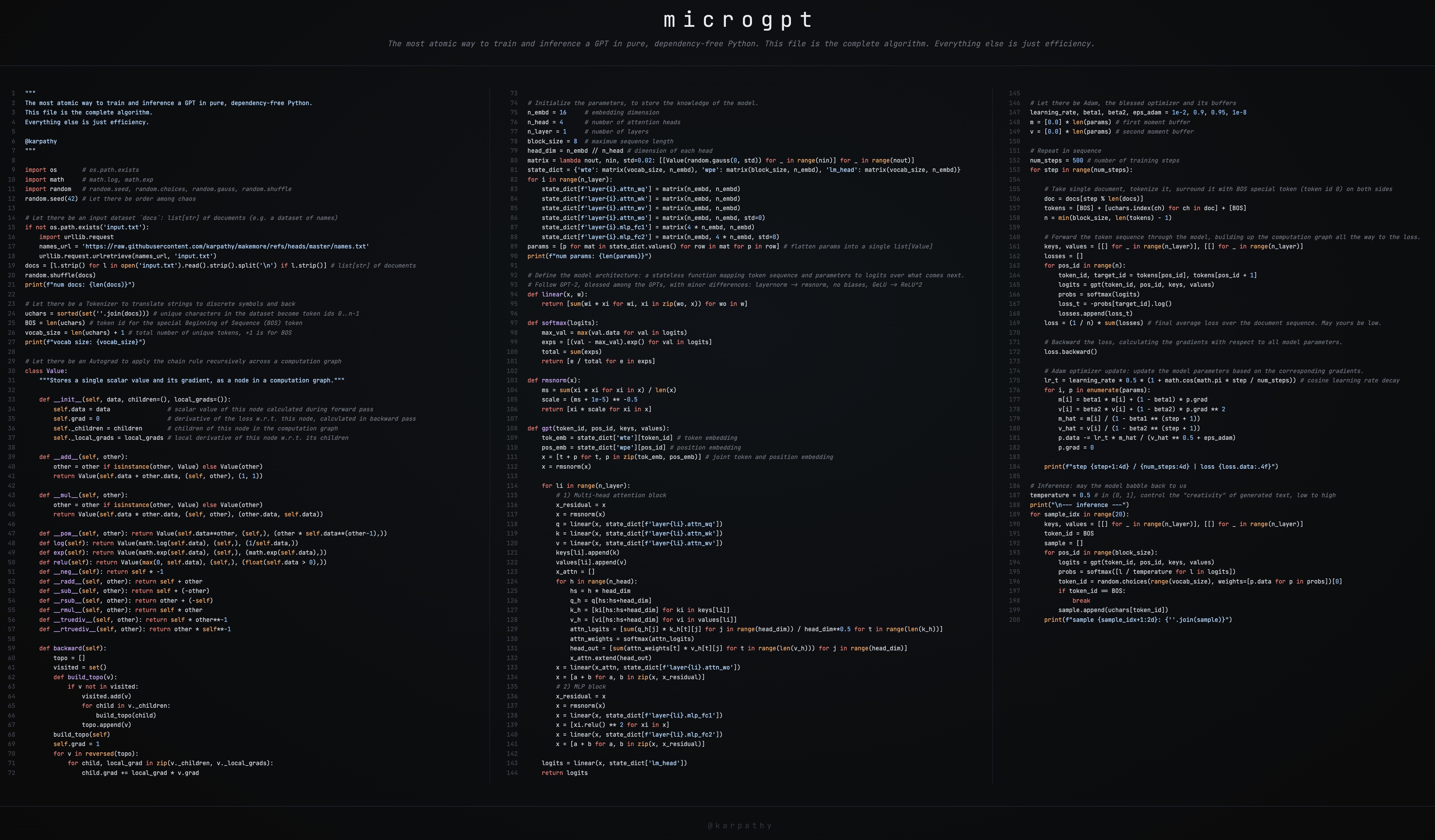
This is a brief guide to my new art project microgpt, a single file of 200 lines of pure Python with no dependencies that trains and inferences a GPT. This file contains the full algorithmic content of what is needed: dataset of documents, tokenizer, autograd engine, a GPT-2-like neural network architecture, the Adam optimizer, training loop, and inference loop. Everything else is just efficiency. I cannot simplify this any further. This script is the culmination of multiple projects (micrograd, makemore, nanogpt, etc.) and a decade-long obsession to simplify LLMs to their bare essentials, and I think it is beautiful 🥹. It even breaks perfectly across 3 columns:
Where to find it:
- This GitHub gist has the full source code: microgpt.py
- It’s also available on this web page: https://karpathy.ai/microgpt.html
- Also available as a Google Colab notebook
The following is my guide on stepping an interested reader through the code.
Dataset
The fuel of large language models is a stream of text data, optionally separated into a set of documents. In production-grade applications, each document would be an internet web page but for microgpt we use a simpler example of 32,000 names, one per line:
# Let there be an input dataset `docs`: list[str] of documents (e.g. a dataset of names)
if not os.path.exists('input.txt'):
    import urllib.request
    names_url = 'https://raw.githubusercontent.com/karpathy/makemore/refs/heads/master/names.txt'
    urllib.request.urlretrieve(names_url, 'input.txt')
docs = [l.strip() for l in open('input.txt').read().strip().split('\n') if l.strip()] # list[str] of documents
random.shuffle(docs)
print(f"num docs: {len(docs)}")
The dataset looks like this. Each name is a document:
emma
olivia
ava
isabella
sophia
charlotte
mia
amelia
harper
... (~32,000 names follow)
The goal of the model is to learn the patterns in the data and then generate similar new documents that share the statistical patterns within. As a preview, by the end of the script our model will generate (“hallucinate”!) new, plausible-sounding names. Skipping ahead, we’ll get:
sample  1: kamon
sample  2: ann
sample  3: karai
sample  4: jaire
sample  5: vialan
sample  6: karia
sample  7: yeran
sample  8: anna
sample  9: areli
sample 10: kaina
sample 11: konna
sample 12: keylen
sample 13: liole
sample 14: alerin
sample 15: earan
sample 16: lenne
sample 17: kana
sample 18: lara
sample 19: alela
sample 20: anton
It doesn’t look like much, but from the perspective of a model like ChatGPT, your conversation with it is just a funny looking “document”. When you initialize the document with your prompt, the model’s response from its perspective is just a statistical document completion.
Tokenizer
Under the hood, neural networks work with numbers, not characters, so we need a way to convert text into a sequence of integer token ids and back. Production tokenizers like tiktoken (used by GPT-4) operate on chunks of characters for efficiency, but the simplest possible tokenizer just assigns one integer to each unique character in the dataset:
# Let there be a Tokenizer to translate strings to discrete symbols and back
uchars = sorted(set(''.join(docs))) # unique characters in the dataset become token ids 0..n-1
BOS = len(uchars) # token id for the special Beginning of Sequence (BOS) token
vocab_size = len(uchars) + 1 # total number of unique tokens, +1 is for BOS
print(f"vocab size: {vocab_size}")
In the code above, we collect all unique characters across the dataset (which are just all the lowercase letters a-z), sort them, and each letter gets an id by its index. Note that the integer values themselves have no meaning at all; each token is just a separate discrete symbol. Instead of 0, 1, 2 they might as well be different emoji. In addition, we create one more special token called BOS (Beginning of Sequence), which acts as a delimiter: it tells the model “a new document starts/ends here”. Later during training, each document gets wrapped with BOS on both sides: [BOS, e, m, m, a, BOS]. The model learns that BOS initates a new name, and that another BOS ends it. Therefore, we have a final vocavulary of 27 (26 possible lowercase characters a-z and +1 for the BOS token).
Autograd
Training a neural network requires gradients: for each parameter in the model, we need to know “if I nudge this number up a little, does the loss go up or down, and by how much?”. The computation graph has many inputs (the model parameters and the input tokens) but funnels down to a single scalar output: the loss (we’ll define exactly what the loss is below). Backpropagation starts at that single output and works backwards through the graph, computing the gradient of the loss with respect to every input. It relies on the chain rule from calculus. In production, libraries like PyTorch handle this automatically. Here, we implement it from scratch in a single class called Value:
class Value:
    __slots__ = ('data', 'grad', '_children', '_local_grads')

    def __init__(self, data, children=(), local_grads=()):
        self.data = data                # scalar value of this node calculated during forward pass
        self.grad = 0                   # derivative of the loss w.r.t. this node, calculated in backward pass
        self._children = children       # children of this node in the computation graph
        self._local_grads = local_grads # local derivative of this node w.r.t. its children

    def __add__(self, other):
        other = other if isinstance(other, Value) else Value(other)
        return Value(self.data + other.data, (self, other), (1, 1))

    def __mul__(self, other):
        other = other if isinstance(other, Value) else Value(other)
        return Value(self.data * other.data, (self, other), (other.data, self.data))

    def __pow__(self, other): return Value(self.data**other, (self,), (other * self.data**(other-1),))
    def log(self): return Value(math.log(self.data), (self,), (1/self.data,))
    def exp(self): return Value(math.exp(self.data), (self,), (math.exp(self.data),))
    def relu(self): return Value(max(0, self.data), (self,), (float(self.data > 0),))
    def __neg__(self): return self * -1
    def __radd__(self, other): return self + other
    def __sub__(self, other): return self + (-other)
    def __rsub__(self, other): return other + (-self)
    def __rmul__(self, other): return self * other
    def __truediv__(self, other): return self * other**-1
    def __rtruediv__(self, other): return other * self**-1

    def backward(self):
        topo = []
        visited = set()
        def build_topo(v):
            if v not in visited:
                visited.add(v)
                for child in v._children:
                    build_topo(child)
                topo.append(v)
        build_topo(self)
        self.grad = 1
        for v in reversed(topo):
            for child, local_grad in zip(v._children, v._local_grads):
                child.grad += local_grad * v.grad
I realize that this is the most mathematically and algorithmically intense part and I have a 2.5 hour video on it: micrograd video. Briefly, a Value wraps a single scalar number (.data) and tracks how it was computed. Think of each operation as a little lego block: it takes some inputs, produces an output (the forward pass), and it knows how its output would change with respect to each of its inputs (the local gradient). That’s all the information autograd needs from each block. Everything else is just the chain rule, stringing the blocks together.
Every time you do math with Value objects (add, multiply, etc.), the result is a new Value that remembers its inputs (_children) and the local derivative of that operation (_local_grads). For example, __mul__ records that \(\frac{\partial(a \cdot b)}{\partial a} = b\) and \(\frac{\partial(a \cdot b)}{\partial b} = a\). The full set of lego blocks:
| Operation | Forward | Local gradients |
|---|---|---|
a + b |
\(a + b\) | \(\frac{\partial}{\partial a} = 1, \quad \frac{\partial}{\partial b} = 1\) |
a * b |
\(a \cdot b\) | \(\frac{\partial}{\partial a} = b, \quad \frac{\partial}{\partial b} = a\) |
a ** n |
\(a^n\) | \(\frac{\partial}{\partial a} = n \cdot a^{n-1}\) |
log(a) |
\(\ln(a)\) | \(\frac{\partial}{\partial a} = \frac{1}{a}\) |
exp(a) |
\(e^a\) | \(\frac{\partial}{\partial a} = e^a\) |
relu(a) |
\(\max(0, a)\) | \(\frac{\partial}{\partial a} = \mathbf{1}_{a > 0}\) |
The backward() method walks this graph in reverse topological order (starting from the loss, ending at the parameters), applying the chain rule at each step. If the loss is \(L\) and a node \(v\) has a child \(c\) with local gradient \(\frac{\partial v}{\partial c}\), then:
This looks a bit scary if you’re not comfortable with your calculus, but this is literally just multiplying two numbers in an intuitive way. One way to see it looks as follows: “If a car travels twice as fast as a bicycle and the bicycle is four times as fast as a walking man, then the car travels 2 x 4 = 8 times as fast as the man.” The chain rule is the same idea: you multiply the rates of change along the path.
We kick things off by setting self.grad = 1 at the loss node, because \(\frac{\partial L}{\partial L} = 1\): the loss’s rate of change with respect to itself is trivially 1. From there, the chain rule just multiplies local gradients along every path back to the parameters.
Note the += (accumulation, not assignment). When a value is used in multiple places in the graph (i.e. the graph branches), gradients flow back along each branch independently and must be summed. This is a consequence of the multivariable chain rule: if \(c\) contributes to \(L\) through multiple paths, the total derivative is the sum of contributions from each path.
After backward() completes, every Value in the graph has a .grad containing \(\frac{\partial L}{\partial v}\), which tells us how the final loss would change if we nudged that value.
Here’s a concrete example. Note that a is used twice (the graph branches), so its gradient is the sum of both paths:
a = Value(2.0)
b = Value(3.0)
c = a * b       # c = 6.0
L = c + a       # L = 8.0
L.backward()
print(a.grad)   # 4.0 (dL/da = b + 1 = 3 + 1, via both paths)
print(b.grad)   # 2.0 (dL/db = a = 2)
This is exactly what PyTorch’s .backward() gives you:
import torch
a = torch.tensor(2.0, requires_grad=True)
b = torch.tensor(3.0, requires_grad=True)
c = a * b
L = c + a
L.backward()
print(a.grad)   # tensor(4.)
print(b.grad)   # tensor(2.)
This is the same algorithm that PyTorch’s loss.backward() runs, just on scalars instead of tensors (arrays of scalars) - algorithmically identical, significantly smaller and simpler, but of course a lot less efficient.
Let’s spell what the .backward() gives us above. Autograd calculated that if L = a*b + a, and a=2 and b=3, then a.grad = 4.0 is telling us about the local influence of a on L. If you wiggle the inmput a, in what direction is L changing? Here, the derivative of L w.r.t. a is 4.0, meaning that if we increase a by a tiny amount (say 0.001), L would increase by about 4x that (0.004). Similarly, b.grad = 2.0 means the same nudge to b would increase L by about 2x that (0.002). In other words, these gradients tell us the direction (positive or negative depending on the sign), and the steepness (the magnitude) of the influence of each individual input on the final output (the loss). This then allows us to interately nudge the parameters of our neural network to lower the loss, and hence improve its predictions.
Parameters
The parameters are the knowledge of the model. They are a large collection of floating point numbers (wrapped in Value for autograd) that start out random and are iteratively optimized during training. The exact role of each parameter will make more sense once we define the model architecture below, but for now we just need to initialize them:
n_embd = 16     # embedding dimension
n_head = 4      # number of attention heads
n_layer = 1     # number of layers
block_size = 16 # maximum sequence length
head_dim = n_embd // n_head # dimension of each head
matrix = lambda nout, nin, std=0.08: [[Value(random.gauss(0, std)) for _ in range(nin)] for _ in range(nout)]
state_dict = {'wte': matrix(vocab_size, n_embd), 'wpe': matrix(block_size, n_embd), 'lm_head': matrix(vocab_size, n_embd)}
for i in range(n_layer):
    state_dict[f'layer{i}.attn_wq'] = matrix(n_embd, n_embd)
    state_dict[f'layer{i}.attn_wk'] = matrix(n_embd, n_embd)
    state_dict[f'layer{i}.attn_wv'] = matrix(n_embd, n_embd)
    state_dict[f'layer{i}.attn_wo'] = matrix(n_embd, n_embd)
    state_dict[f'layer{i}.mlp_fc1'] = matrix(4 * n_embd, n_embd)
    state_dict[f'layer{i}.mlp_fc2'] = matrix(n_embd, 4 * n_embd)
params = [p for mat in state_dict.values() for row in mat for p in row]
print(f"num params: {len(params)}")
Each parameter is initialized to a small random number drawn from a Gaussian distribution. The state_dict organizes them into named matrices (borrowing PyTorch’s terminology): embedding tables, attention weights, MLP weights, and a final output projection. We also flatten all parameters into a single list params so the optimizer can loop over them later. In our tiny model this comes out to 4,192 parameters. GPT-2 had 1.6 billion, and modern LLMs have hundreds of billions.
Architecture
The model architecture is a stateless function: it takes a token, a position, the parameters, and the cached keys/values from previous positions, and returns logits (scores) over what token the model things should come next in the sequence. We follow GPT-2 with minor simplifications: RMSNorm instead of LayerNorm, no biases, and ReLU instead of GeLU. First, three small helper functions:
def linear(x, w):
    return [sum(wi * xi for wi, xi in zip(wo, x)) for wo in w]
linear is a matrix-vector multiply. It takes a vector x and a weight matrix w, and computes one dot product per row of w. This is the fundamental building block of neural networks: a learned linear transformation.
def softmax(logits):
    max_val = max(val.data for val in logits)
    exps = [(val - max_val).exp() for val in logits]
    total = sum(exps)
    return [e / total for e in exps]
softmax converts a vector of raw scores (logits), which can range from \(-\infty\) to \(+\infty\), into a probability distribution: all values end up in \([0, 1]\) and sum to 1. We subtract the max first for numerical stability (it doesn’t change the result mathematically, but prevents overflow in exp).
def rmsnorm(x):
    ms = sum(xi * xi for xi in x) / len(x)
    scale = (ms + 1e-5) ** -0.5
    return [xi * scale for xi in x]
rmsnorm (Root Mean Square Normalization) rescales a vector so its values have unit root-mean-square. This keeps activations from growing or shrinking as they flow through the network, which stabilizes training. It’s a simpler variant of the LayerNorm used in the original GPT-2.
Now the model itself:
def gpt(token_id, pos_id, keys, values):
    tok_emb = state_dict['wte'][token_id] # token embedding
    pos_emb = state_dict['wpe'][pos_id] # position embedding
    x = [t + p for t, p in zip(tok_emb, pos_emb)] # joint token and position embedding
    x = rmsnorm(x)

    for li in range(n_layer):
        # 1) Multi-head attention block
        x_residual = x
        x = rmsnorm(x)
        q = linear(x, state_dict[f'layer{li}.attn_wq'])
        k = linear(x, state_dict[f'layer{li}.attn_wk'])
        v = linear(x, state_dict[f'layer{li}.attn_wv'])
        keys[li].append(k)
        values[li].append(v)
        x_attn = []
        for h in range(n_head):
            hs = h * head_dim
            q_h = q[hs:hs+head_dim]
            k_h = [ki[hs:hs+head_dim] for ki in keys[li]]
            v_h = [vi[hs:hs+head_dim] for vi in values[li]]
            attn_logits = [sum(q_h[j] * k_h[t][j] for j in range(head_dim)) / head_dim**0.5 for t in range(len(k_h))]
            attn_weights = softmax(attn_logits)
            head_out = [sum(attn_weights[t] * v_h[t][j] for t in range(len(v_h))) for j in range(head_dim)]
            x_attn.extend(head_out)
        x = linear(x_attn, state_dict[f'layer{li}.attn_wo'])
        x = [a + b for a, b in zip(x, x_residual)]
        # 2) MLP block
        x_residual = x
        x = rmsnorm(x)
        x = linear(x, state_dict[f'layer{li}.mlp_fc1'])
        x = [xi.relu() for xi in x]
        x = linear(x, state_dict[f'layer{li}.mlp_fc2'])
        x = [a + b for a, b in zip(x, x_residual)]

    logits = linear(x, state_dict['lm_head'])
    return logits
The function processes one token (of id token_id) at a specific position in time (pos_id), and some context
from the previous iterations summarized by the activations in keys and values, known as the KV Cache. Here’s what happens step by step:
Embeddings. The neural network can’t process a raw token id like 5 directly. It can only work with vectors (lists of numbers). So we associate a learned vector with each possible token, and feed that in as its neural signature. The token id and position id each look up a row from their respective embedding tables (wte and wpe). These two vectors are added together, giving the model a representation that encodes both what the token is and where it is in the sequence. Modern LLMs usually skip the position embedding and introduce other relative-based positioning schemes, e.g. RoPE.
Attention block. The current token is projected into three vectors: a query (Q), a key (K), and a value (V). Intuitively, the query says “what am I looking for?”, the key says “what do I contain?”, and the value says “what do I offer if selected?”. For example, in the name “emma”, when the model is at the second “m” and trying to predict what comes next, it might learn a query like “what vowels appeared recently?” The earlier “e” would have a key that matches this query well, so it gets a high attention weight, and its value (information about being a vowel) flows into the current position. The key and value are appended to the KV cache so previous positions are available. Each attention head computes dot products between its query and all cached keys (scaled by \(\sqrt{d_{head}}\)), applies softmax to get attention weights, and takes a weighted sum of the cached values. The outputs of all heads are concatenated and projected through attn_wo. It’s worth emphasizing that the Attention block is the exact and only place where a token at position t gets to “look” at tokens in the past 0..t-1. Attention is a token communication mechanism.
MLP block. MLP is short for “multilayer perceptron”, it is a two-layer feed-forward network: project up to 4x the embedding dimension, apply ReLU, project back down. This is where the model does most of its “thinking” per position. Unlike attention, this computation is fully local to time t. The Transformer intersperses communication (Attention) with computation (MLP).
Residual connections. Both the attention and MLP blocks add their output back to their input (x = [a + b for ...]). This lets gradients flow directly through the network and makes deeper models trainable.
Output. The final hidden state is projected to vocabulary size by lm_head, producing one logit per token in the vocabulary. In our case, that’s just 27 numbers. Higher logit = the model thinks that corresponding token is more likely to come next.
You might notice that we’re using a KV cache during training, which is unusual. People typically associate the KV cache with inference only. But the KV cache is conceptually always there, even during training. In production implementations, it’s just hidden inside the highly vectorized attention computation that processes all positions in the sequence simultaneously. Since microgpt processes one token at a time (no batch dimension, no parallel time steps), we build the KV cache explicitly. And unlike the typical inference setting where the KV cache holds detached tensors, here the cached keys and values are live Value nodes in the computation graph, so we actually backpropagate through them.
Training loop
Now we wire everything together. The training loop repeatedly: (1) picks a document, (2) runs the model forward over its tokens, (3) computes a loss, (4) backpropagates to get gradients, and (5) updates the parameters.
# Let there be Adam, the blessed optimizer and its buffers
learning_rate, beta1, beta2, eps_adam = 0.01, 0.85, 0.99, 1e-8
m = [0.0] * len(params) # first moment buffer
v = [0.0] * len(params) # second moment buffer

# Repeat in sequence
num_steps = 1000 # number of training steps
for step in range(num_steps):

    # Take single document, tokenize it, surround it with BOS special token on both sides
    doc = docs[step % len(docs)]
    tokens = [BOS] + [uchars.index(ch) for ch in doc] + [BOS]
    n = min(block_size, len(tokens) - 1)

    # Forward the token sequence through the model, building up the computation graph all the way to the loss.
    keys, values = [[] for _ in range(n_layer)], [[] for _ in range(n_layer)]
    losses = []
    for pos_id in range(n):
        token_id, target_id = tokens[pos_id], tokens[pos_id + 1]
        logits = gpt(token_id, pos_id, keys, values)
        probs = softmax(logits)
        loss_t = -probs[target_id].log()
        losses.append(loss_t)
    loss = (1 / n) * sum(losses) # final average loss over the document sequence. May yours be low.

    # Backward the loss, calculating the gradients with respect to all model parameters.
    loss.backward()

    # Adam optimizer update: update the model parameters based on the corresponding gradients.
    lr_t = learning_rate * (1 - step / num_steps) # linear learning rate decay
    for i, p in enumerate(params):
        m[i] = beta1 * m[i] + (1 - beta1) * p.grad
        v[i] = beta2 * v[i] + (1 - beta2) * p.grad ** 2
        m_hat = m[i] / (1 - beta1 ** (step + 1))
        v_hat = v[i] / (1 - beta2 ** (step + 1))
        p.data -= lr_t * m_hat / (v_hat ** 0.5 + eps_adam)
        p.grad = 0

    print(f"step {step+1:4d} / {num_steps:4d} | loss {loss.data:.4f}")
Let’s walk through each piece:
Tokenization. Each training step picks one document and wraps it with BOS on both sides: the name “emma” becomes [BOS, e, m, m, a, BOS]. The model’s job is to predict each next token given the tokens before it.
Forward pass and loss. We feed the tokens through the model one at a time, building up the KV cache as we go. At each position, the model outputs 27 logits, which we convert to probabilities via softmax. The loss at each position is the negative log probability of the correct next token: \(-\log p(\text{target})\). This is called the cross-entropy loss. Intuitively, the loss measures the degree of misprediction: how surprised the model is by what actually comes next. If the model assigns probability 1.0 to the correct token, it is not surprised at all and the loss is 0. If it assigns probability close to 0, the model is very surprised and the loss goes to \(+\infty\). We average the per-position losses across the document to get a single scalar loss.
Backward pass. One call to loss.backward() runs backpropagation through the entire computation graph, from the loss all the way back through softmax, the model, and into every parameter. After this, each parameter’s .grad tells us how to change it to reduce the loss.
Adam optimizer. We could just do p.data -= lr * p.grad (gradient descent), but Adam is smarter. It maintains two running averages per parameter: m tracks the mean of recent gradients (momentum, like a rolling ball), and v tracks the mean of recent squared gradients (adapting the learning rate per parameter). The m_hat and v_hat are bias corrections that account for the fact that m and v are initialized to zero and need a warmup. The learning rate decays linearly over training. After updating, we reset .grad = 0 for the next step.
Over 1,000 steps the loss decreases from around 3.3 (random guessing among 27 tokens: \(-\log(1/27) \approx 3.3\)) down to around 2.37. Lower is better, and the lowest possible is 0 (perfect predictions), so there’s still room to improve, but the model is clearly learning the statistical patterns of names.
Inference
Once training is done, we can sample new names from the model. The parameters are frozen and we just run the forward pass in a loop, feeding each generated token back as the next input:
temperature = 0.5 # in (0, 1], control the "creativity" of generated text, low to high
print("\n--- inference (new, hallucinated names) ---")
for sample_idx in range(20):
    keys, values = [[] for _ in range(n_layer)], [[] for _ in range(n_layer)]
    token_id = BOS
    sample = []
    for pos_id in range(block_size):
        logits = gpt(token_id, pos_id, keys, values)
        probs = softmax([l / temperature for l in logits])
        token_id = random.choices(range(vocab_size), weights=[p.data for p in probs])[0]
        if token_id == BOS:
            break
        sample.append(uchars[token_id])
    print(f"sample {sample_idx+1:2d}: {''.join(sample)}")
We start each sample with the BOS token, which tells the model “begin a new name”. The model produces 27 logits, we convert them to probabilities, and we randomly sample one token according to those probabilities. That token gets fed back in as the next input, and we repeat until the model produces BOS again (meaning “I’m done”) or we hit the maximum sequence length.
The temperature parameter controls randomness. Before softmax, we divide the logits by the temperature. A temperature of 1.0 samples directly from the model’s learned distribution. Lower temperatures (like 0.5 here) sharpen the distribution, making the model more conservative and likely to pick its top choices. A temperature approaching 0 would always pick the single most likely token (greedy decoding). Higher temperatures flatten the distribution and produce more diverse but potentially less coherent output.
Run it
All you need is Python (no pip install, no dependencies):
python train.py
The script takes about 1 minute to run on my macbook. You’ll see the loss printed at each step:
train.py
num docs: 32033
vocab size: 27
num params: 4192
step    1 / 1000 | loss 3.3660
step    2 / 1000 | loss 3.4243
step    3 / 1000 | loss 3.1778
step    4 / 1000 | loss 3.0664
step    5 / 1000 | loss 3.2209
step    6 / 1000 | loss 2.9452
step    7 / 1000 | loss 3.2894
step    8 / 1000 | loss 3.3245
step    9 / 1000 | loss 2.8990
step   10 / 1000 | loss 3.2229
step   11 / 1000 | loss 2.7964
step   12 / 1000 | loss 2.9345
step   13 / 1000 | loss 3.0544
...
Watch it go down from ~3.3 (random) toward ~2.37. The lower this number is, the better the network’s predictions already were about what token comes next in the sequence. At the end of training, the knowledge of the stastical patterns of the training token sequences is distilled in the model parameters. Fixing these parameters, we can now generate new, hallucinated names. You’ll see (again):
sample  1: kamon
sample  2: ann
sample  3: karai
sample  4: jaire
sample  5: vialan
sample  6: karia
sample  7: yeran
sample  8: anna
sample  9: areli
sample 10: kaina
sample 11: konna
sample 12: keylen
sample 13: liole
sample 14: alerin
sample 15: earan
sample 16: lenne
sample 17: kana
sample 18: lara
sample 19: alela
sample 20: anton
As an alternative to running the script on your computer, you may try to run it directly on this Google Colab notebook and ask Gemini questions about it. Try playing with the script! You can try a different dataset. Or you can train for longer (increase num_steps) or increase the size of the model to get increasingly better results.
Real stuff
microgpt contains the complete algorithmic essence of training and running a GPT. But between this and a production LLM like ChatGPT, there is a long list of things that change. None of them alter the core algorithm and the overall layout, but they are what makes it actually work at scale. Walking through the same sections in order:
Data. Instead of 32K short names, production models train on trillions of tokens of internet text: web pages, books, code, etc. The data is deduplicated, filtered for quality, and carefully mixed across domains.
Tokenizer. Instead of single characters, production models use subword tokenizers like BPE (Byte Pair Encoding), which learn to merge frequently co-occurring character sequences into single tokens. Common words like “the” become a single token, rare words get broken into pieces. This gives a vocabulary of ~100K tokens and is much more efficient because the model sees more content per position.
Autograd. microgpt operates on scalar Value objects in pure Python. Production systems use tensors (large multi-dimensional arrays of numbers) and run on GPUs/TPUs that perform billions of floating point operations per second. Libraries like PyTorch handle the autograd over tensors, and CUDA kernels like FlashAttention fuse multiple operations for speed. The math is identical, just corresponds to many scalars processed in parallel.
Architecture. microgpt has 4,192 parameters. GPT-4 class models have hundreds of billions. Overall it’s a very similar looking Transformer neural network, just much wider (embedding dimensions of 10,000+) and much deeper (100+ layers). Modern LLMs also incorporate a few more types of lego blocks and change their orders around: Examples include RoPE (Rotary Position Embeddings) instead of learned position embeddings, GQA (Grouped Query Attention) to reduce KV cache size, gated linear activations instead of ReLU, Mixture of Experts (MoE) layers, etc. But the core structure of Attention (communication) and MLP (computation) interspersed on a residual stream is well-preserved.
Training. Instead of one document per step, production training uses large batches (millions of tokens per step), gradient accumulation, mixed precision (float16/bfloat16), and careful hyperparameter tuning. Training a frontier model takes thousands of GPUs running for months.
Optimization. microgpt uses Adam with a simple linear learning rate decay and that’s about it. At scale, optimization becomes its own discipline. Models train in reduced precision (bfloat16 or even fp8) and across large GPU clusters for efficiency, which introduces its own numerical challenges. The optimizer settings (learning rate, weight decay, beta parameters, warmup schedule, decay schedule) must be tuned precisely, and the right values depend on model size, batch size, and dataset composition. Scaling laws (e.g. Chinchilla) guide how to allocate a fixed compute budget between model size and number of training tokens. Getting any of these details wrong at scale can waste millions of dollars of compute, so teams run extensive smaller-scale experiments to predict the right settings before committing to a full training run.
Post-training. The base model that comes out of training (called the “pretrained” model) is a document completer, not a chatbot. Turning it into ChatGPT happens in two stages. First, SFT (Supervised Fine-Tuning): you simply swap the documents for curated conversations and keep training. Algorithmically, nothing changes. Second, RL (Reinforcement Learning): the model generates responses, they get scored (by humans, another “judge” model, or an algorithm), and the model learns from that feedback. Fundamentally, the model is still training on documents, but those documents are now made up of tokens coming from the model itself.
Inference. Serving a model to millions of users requires its own engineering stack: batching requests together, KV cache management and paging (vLLM, etc.), speculative decoding for speed, quantization (running in int8/int4 instead of float16) to reduce memory, and distributing the model across multiple GPUs. Fundamentally, we are still predicting the next token in the sequence but with a lot of engineering spent on making it faster.
All of these are important engineering and research contributions but if you understand microgpt, you understand the algorithmic essence.
FAQ
Does the model “understand” anything? That’s a philosophical question, but mechanically: no magic is happening. The model is a big math function that maps input tokens to a probability distribution over the next token. During training, the parameters are adjusted to make the correct next token more probable. Whether this constitutes “understanding” is up to you, but the mechanism is fully contained in the 200 lines above.
Why does it work? The model has thousands of adjustable parameters, and the optimizer nudges them a tiny bit each step to make the loss go down. Over many steps, the parameters settle into values that capture the statistical regularities of the data. For names, this means things like: names often start with consonants, “qu” tends to appear together, names rarely have three consonants in a row, etc. The model doesn’t learn explicit rules, it learns a probability distribution that happens to reflect them.
How is this related to ChatGPT? ChatGPT is this same core loop (predict next token, sample, repeat) scaled up enormously, with post-training to make it conversational. When you chat with it, the system prompt, your message, and its reply are all just tokens in a sequence. The model is completing the document one token at a time, same as microgpt completing a name.
What’s the deal with “hallucinations”? The model generates tokens by sampling from a probability distribution. It has no concept of truth, it only knows what sequences are statistically plausible given the training data. microgpt “hallucinating” a name like “karia” is the same phenomenon as ChatGPT confidently stating a false fact. Both are plausible-sounding completions that happen not to be real.
Why is it so slow? microgpt processes one scalar at a time in pure Python. A single training step takes seconds. The same math on a GPU processes millions of scalars in parallel and runs orders of magnitude faster.
Can I make it generate better names? Yes. Train longer (increase num_steps), make the model bigger (n_embd, n_layer, n_head), or use a larger dataset. These are the same knobs that matter at scale.
What if I change the dataset? The model will learn whatever patterns are in the data. Swap in a file of city names, Pokemon names, English words, or short poems, and the model will learn to generate those instead. The rest of the code doesn’t need to change.